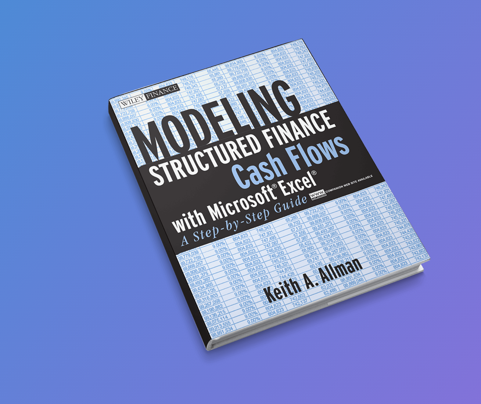
Modeling Structured Finance Cash Flows
Enstruct’s principal’s debut book on modeling structured finance securities. It is an easily accessible text that takes a reader through every component of the analytical process for structured finance assets. Readers build their modeling experience in each chapter through Model Builder exercises, which culminate into a final, consolidated model. Included with this text is download access with the Excel versions of the Model Builder exercises and the complete model.
Errata
Course Outline
p. 31 Step 14 instructs the reader to enter 1.50% for the margin, however the download access models leave this field blank. The corrected model files should have 1.50% entered for the margin to begin with.
p. 31 Step 10 instructs the reader to name a cell Age1. This will be fine for versions of Excel up to 2003, however it will not work for Excel 2007.
p.38 Step 14 the final F6 of the formula should be F6-AssetMarg1
p.38 the final formula in step 14 is created in such a way that the lifetime cap entered on the Assumptions sheet will never be exceeded, INCLUSIVE of the margin. A more consistent implementation with the wording of the book is the following formula:
=IF(AssetIntType1=”Fixed”,AssetFxdRate1,IF(A7=1,OFFSET(Vectors!$D$6,A7,MATCH(AssetFltIndx1,lstInterestRates,0)),I
F(MOD($A7,AssetRateReset1)=0,MAX(MIN(OFFSET(Vectors!$D$6,A7,MATCH(AssetFltIndx1,lstInterestRates,0)),(F6-AssetMarg1)+AssetPdCapFl1,AssetLifeCap1),(F6-AssetMarg1)-AssetPdCapFl1,AssetLifeFloor1-AssetMarg1),F6-AssetMarg1)))+AssetMarg1
This formula only implements the lifetime cap on the index and then adds the margin.
p.38-39 Step 15 instructs the reader to enter a formula for the periodic payment. Originally the model was only going to be set to a fixed rate system, but to be more flexible it was created with a floating rate system and the text explains floating rate functionality. However, the complete formula was never picked up in the Model Builder, nor the text. The proper notional payment formula should read:
=IF(J6<=G6,H7+E7,IF(AssetIntType1=”Fixed”,-PMT(AssetFxdRate1*IF(A7=1,$C$7,$C$8),OrgTerm1,
AssetOrgBal1),-PMT(F7*C7,OrgTerm1-A6,E7)))
Notice that there is now an IF to define the Fixed versus Floating state. In the fixed state we assume the fixed rate and whatever the starting day count factor is. Most likely this will be 30/360, but be careful when using actual because it should represent what the loan was originated with. The second part requires the rate and day factor system to change over time (no dollar signs) AND that the term and balance change. This will create a variable payment within the terms specified.
p.49 Step 3 clear cells C7:AA7 instead of A7:AA7.
General – the named cell AssetTerm1 is used in the book and some Model Builder exercises. At some point it was changed to OrgTerm1, which is reflected in the final model. The names refer to the same thing, so either will do, just make sure to be consistent.
p. 54 Step 6 should describe labeling row 4, not row 5.
I. Time Value of Money Functions
II. Mathematical/Statistical Functions
III. Logical Functions
IV. Lookup Functions
V. Naming Ranges/Data Validation Lists
VI. Function Combinations
Time Value of Money Functions
Mathematical/Statistical Functions
Logical Functions
Lookup Functions
Naming Ranges/ Data Validation Lists
p. 62 Step 4 should instruct the reader to insert 23 in cell A69, not B68.
p. 67 The raw data file from Model Builder 4.2 – Raw Data has three additional months of data for every period. This can be deleted.
p. 68 Step 2 is unnecessary since the data is already copied down.
p. 76 Step 2 and 3 instruct the reader to enter multiple labels on rows 4 and 5. In the Model Builder and completed model these labels appear on rows 3 and 4. To make the model easier to tie to the completed model label use rows 3 and 4 for the labels.
p.78 Step 7 could confuse readers trying to get to the 3.33333333%. When entering =100/30 you will want to make sure this is a percent by modifying the formula to =(100/30)%. Or you could simply take the original formula and divide by 100.
p. 82 Step 13 instructs the reader to enter the formula =(L7-N7)*(1-O7/O6). This formula needs to be cleaned up in case the current balance is 0. The correct formula should be =IF(L7<=0,0,(L7-N7)*(1-O7/O6).
I. Overview of a Scenario Selector
II. Specific Scenario Selector Setup & Use
Exercise: Scenario Selectors
p. 122 Step 16 instructs the reader to modify the formula by adding AX7+BH7-AV7 to the MIN statement in the beginning. This is correct, but the original AX7 must be removed. The final formula for AZ7 should read: =IF(OR(Z7, AB7,AC7),MIN(AX7+BH7-AV7,CB6),IF(LiabPrinType1=”Sequential”,MIN((N7+Q7+R7),CB6),MIN((N7+Q7+R7)*LiabAdvRate1,CB6)))
I. Overview of Dates and Timing Set Up
II. Specific Date and Timing Functions and Organization
Exercise: Dates & Timing
p.134 The formula for modified duration in the book and Project Model Builder is:=1/((1+E5/12))*(SUMPRODUCT(E16:E375,$A$16:$A$375)/(12*E4)). The correct formula should reference the BEY, not the monthly yield. To do this simply change the formula to:=1/((1+E7/12))*(SUMPRODUCT(E16:E375,$A$16:$A$375)/(12*E4))
The waterfall in the example model created from this text is set to change by selecting different periodicities. However, the Analytics sheet and the Output sheet are set to monthly periodicity. If you would like to make them completely dynamic then you would need to replace the hard coded divisors with divisors from the periodicity references created on the Hidden sheet.
Also related to periodicity there is an error on the Hidden sheet where “Semi Annual” is missing the hypen. This causes a problem when selecting that periodicity because the formula is coded with a hyphen. The periodicity reverts to annual. To correct this make the list the same as the formula, either removing or adding a hyphen where necessary.
On the Output sheet there are a couple of columns where the OFFSET function did not get copied over. This should be copied over for all sections that rely on referencing periods selected by the user on the Inputs sheet.


